Show the code
set.seed(1337)

library("tidymodels")
tidymodels::tidymodels_prefer()Set seed and load packages.
set.seed(1337)
library("tidymodels")
tidymodels::tidymodels_prefer()Load data.
mtcars <- mtcars |>
  as_tibble()
A general use case in statistics is to predict new data given some input data. Endless examples exist, such as predicting the price of a house given the size of the house or predicting the miles pr gallon of a car given the weight of the car. To do so, some model is needed. A wide range of models for predicting data exists. One of the most common models is a linear regression model. Introduced in this chapter is the model called Ordinary Least Squares (OLS).
The general idea is to fit a line to the data, such that the sum of the squared residuals is minimized, hence the name least squares. Residuals are the difference between the actual value and the predicted value of the model.
Another famously used data set is the mtcars. Below is an example of a scatter plot of the miles pr gallon (mpg) vs the weight of the car (wt). By fitting a linear regression model, the goal is to predict the miles pr gallon based on the weight of the car. For an initial guess, the mean of the miles pr gallon is used, shown as the red dashed line. The residuals are the distance between the actual value (dots) and the predicted value (red dashed line). The sum of the squares of the residuals is then used as a measure of how well the model fits the data. As some predicted values are below the actual value, and some values are above, these can counter balance each other, such that the sum of the residuals is 0. To avoid this, the residuals are squared, such that all residuals are positive. Further, by squaring the residuals the bigger residuals have a larger effect on the sum of the residuals squared. Since the goal is to minimize the sum of the residuals squared, the bigger residuals are more important to reduce.
mpg_mean <- mtcars |>
  pull(mpg) |>
  mean()

mtcars |>
  ggplot(aes(x = wt,
             y = mpg)) +
  geom_point(size = 3,
             colour = "steelblue") +
  geom_hline(yintercept = mpg_mean,
             colour = "firebrick",
             linetype = "dashed") +
  labs(title = "Miles pr Gallon vs Weight",
       x = "Weight (1000 lbs)",
       y = "Miles pr Gallon",
       colour = "Miles per gallon") +
  theme(text=element_text(size=13))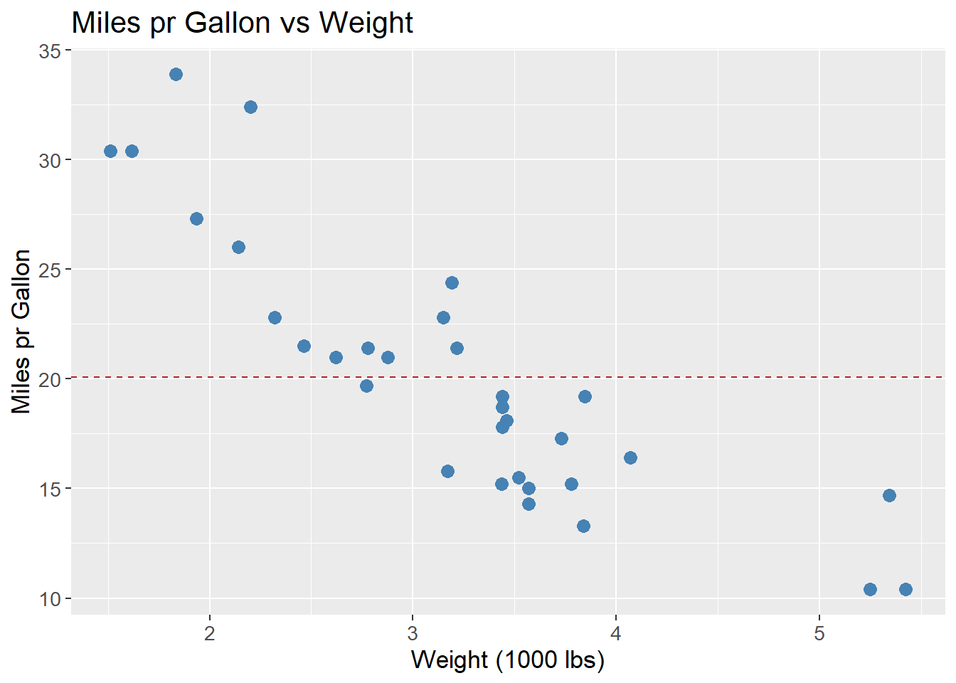
In this simple case, the model is fitting the line to the data by changing the slope and intercept of the line. The combination which minimizes the sum of the squared residuals (SSR) is chosen. This results in a three dimensional space, where the slope and intercept are plotted along the x and y axis, and the sum of the squared residuals are plotted along the z-axis. Some combination of slope and intercept results in a minimum in the 3D plane. This combination can be found by taking the derivative of the sum of the squared residuals with respect to the slope and intercept, and set it equal to zero.
The model can be generalized to more than one feature, such that the model can predict the response based on multiple features. Usually, the simple linear case is written as \(y = ax + b\) where \(a\) is the slope and \(b\) is the intercept. When using multiple features, it is generalized to \(y = \beta_0 + \beta_{1}x_1 + \beta_{2}x_2 + ... + \beta_{n}x_n\). In matrix form it can be written as \(y = X\beta\) where \(X\) is a matrix with \(n\) rows (number of observations) and \(p\) columns (number of features). \(\beta\) is a vector of length \(p\) which includes a parameter for each feature.
As mentioned earlier, the goal is to minimize the sum of the squared residuals. On matrix form, SSR is written as:
\[ SSR = ||y-X\beta||_{2}^{2} \]
Where the subscript 2 denotes the L2 norm, i.e. Euclidean distance. The term \(X\beta\) is the predicted value of the model as we saw from \(y = X\beta\) in the above. SSR is also written as:
\[ SSR = \sum_{i=1}^{n} (y_i - X_{i}\beta)^2 = \sum_{i=1}^{n} (y_i - \hat{y}_i)^2 \]
Where \(\hat{y}_i\) is the predicted value of the model for the \(i\)’th sample. Since the goal is to minimize the SSR, the \(\beta\)s should be chosen such that the SSR is minimized:
\[ \beta_{OLS} = \min_{\beta} SSR = \min_{\beta} ||y-X\beta||_{2}^{2} \]
As mentioned in the above, the \(\beta\)s can be found by taking the derivative of the SSR with respect to \(\beta\) and set it equal to zero. Since this is generalized to multiple features, the gradient is taken with respect to the vector \(\beta\) instead. The equation is then:
\[ \nabla_\beta||y-X\beta||_{2}^{2} = 0 \]
sessioninfo::session_info()─ Session info ───────────────────────────────────────────────────────────────
setting value
version R version 4.3.3 (2024-02-29 ucrt)
os Windows 11 x64 (build 22631)
system x86_64, mingw32
ui RTerm
language (EN)
collate English_United Kingdom.utf8
ctype English_United Kingdom.utf8
tz Europe/Copenhagen
date 2024-05-30
pandoc 3.1.11 @ C:/Program Files/RStudio/resources/app/bin/quarto/bin/tools/ (via rmarkdown)
─ Packages ───────────────────────────────────────────────────────────────────
package * version date (UTC) lib source
backports 1.4.1 2021-12-13 [1] CRAN (R 4.3.1)
broom * 1.0.5 2023-06-09 [1] CRAN (R 4.3.3)
cachem 1.0.8 2023-05-01 [1] CRAN (R 4.3.3)
class 7.3-22 2023-05-03 [2] CRAN (R 4.3.3)
cli 3.6.2 2023-12-11 [1] CRAN (R 4.3.3)
codetools 0.2-19 2023-02-01 [2] CRAN (R 4.3.3)
colorspace 2.1-0 2023-01-23 [1] CRAN (R 4.3.3)
conflicted 1.2.0 2023-02-01 [1] CRAN (R 4.3.3)
data.table 1.15.4 2024-03-30 [1] CRAN (R 4.3.3)
dials * 1.2.1 2024-02-22 [1] CRAN (R 4.3.3)
DiceDesign 1.10 2023-12-07 [1] CRAN (R 4.3.3)
digest 0.6.35 2024-03-11 [1] CRAN (R 4.3.3)
dplyr * 1.1.4 2023-11-17 [1] CRAN (R 4.3.2)
evaluate 0.23 2023-11-01 [1] CRAN (R 4.3.3)
fansi 1.0.6 2023-12-08 [1] CRAN (R 4.3.3)
farver 2.1.1 2022-07-06 [1] CRAN (R 4.3.3)
fastmap 1.1.1 2023-02-24 [1] CRAN (R 4.3.3)
foreach 1.5.2 2022-02-02 [1] CRAN (R 4.3.3)
furrr 0.3.1 2022-08-15 [1] CRAN (R 4.3.3)
future 1.33.2 2024-03-26 [1] CRAN (R 4.3.3)
future.apply 1.11.2 2024-03-28 [1] CRAN (R 4.3.3)
generics 0.1.3 2022-07-05 [1] CRAN (R 4.3.3)
ggplot2 * 3.5.1 2024-04-23 [1] CRAN (R 4.3.3)
globals 0.16.3 2024-03-08 [1] CRAN (R 4.3.3)
glue 1.7.0 2024-01-09 [1] CRAN (R 4.3.3)
gower 1.0.1 2022-12-22 [1] CRAN (R 4.3.1)
GPfit 1.0-8 2019-02-08 [1] CRAN (R 4.3.3)
gtable 0.3.5 2024-04-22 [1] CRAN (R 4.3.3)
hardhat 1.3.1 2024-02-02 [1] CRAN (R 4.3.3)
htmltools 0.5.8.1 2024-04-04 [1] CRAN (R 4.3.3)
htmlwidgets 1.6.4 2023-12-06 [1] CRAN (R 4.3.3)
infer * 1.0.7 2024-03-25 [1] CRAN (R 4.3.3)
ipred 0.9-14 2023-03-09 [1] CRAN (R 4.3.3)
iterators 1.0.14 2022-02-05 [1] CRAN (R 4.3.3)
jsonlite 1.8.8 2023-12-04 [1] CRAN (R 4.3.3)
knitr 1.46 2024-04-06 [1] CRAN (R 4.3.3)
labeling 0.4.3 2023-08-29 [1] CRAN (R 4.3.1)
lattice 0.22-5 2023-10-24 [2] CRAN (R 4.3.3)
lava 1.8.0 2024-03-05 [1] CRAN (R 4.3.3)
lhs 1.1.6 2022-12-17 [1] CRAN (R 4.3.3)
lifecycle 1.0.4 2023-11-07 [1] CRAN (R 4.3.3)
listenv 0.9.1 2024-01-29 [1] CRAN (R 4.3.3)
lubridate 1.9.3 2023-09-27 [1] CRAN (R 4.3.3)
magrittr 2.0.3 2022-03-30 [1] CRAN (R 4.3.3)
MASS 7.3-60.0.1 2024-01-13 [2] CRAN (R 4.3.3)
Matrix 1.6-5 2024-01-11 [2] CRAN (R 4.3.3)
memoise 2.0.1 2021-11-26 [1] CRAN (R 4.3.3)
modeldata * 1.3.0 2024-01-21 [1] CRAN (R 4.3.3)
munsell 0.5.1 2024-04-01 [1] CRAN (R 4.3.3)
nnet 7.3-19 2023-05-03 [2] CRAN (R 4.3.3)
parallelly 1.37.1 2024-02-29 [1] CRAN (R 4.3.3)
parsnip * 1.2.1 2024-03-22 [1] CRAN (R 4.3.3)
pillar 1.9.0 2023-03-22 [1] CRAN (R 4.3.3)
pkgconfig 2.0.3 2019-09-22 [1] CRAN (R 4.3.3)
prodlim 2023.08.28 2023-08-28 [1] CRAN (R 4.3.3)
purrr * 1.0.2 2023-08-10 [1] CRAN (R 4.3.3)
R6 2.5.1 2021-08-19 [1] CRAN (R 4.3.3)
Rcpp 1.0.12 2024-01-09 [1] CRAN (R 4.3.3)
recipes * 1.0.10 2024-02-18 [1] CRAN (R 4.3.3)
rlang 1.1.3 2024-01-10 [1] CRAN (R 4.3.3)
rmarkdown 2.26 2024-03-05 [1] CRAN (R 4.3.3)
rpart 4.1.23 2023-12-05 [2] CRAN (R 4.3.3)
rsample * 1.2.1 2024-03-25 [1] CRAN (R 4.3.3)
rstudioapi 0.16.0 2024-03-24 [1] CRAN (R 4.3.3)
scales * 1.3.0 2023-11-28 [1] CRAN (R 4.3.3)
sessioninfo 1.2.2 2021-12-06 [1] CRAN (R 4.3.3)
survival 3.5-8 2024-02-14 [2] CRAN (R 4.3.3)
tibble * 3.2.1 2023-03-20 [1] CRAN (R 4.3.3)
tidymodels * 1.2.0 2024-03-25 [1] CRAN (R 4.3.3)
tidyr * 1.3.1 2024-01-24 [1] CRAN (R 4.3.3)
tidyselect 1.2.1 2024-03-11 [1] CRAN (R 4.3.3)
timechange 0.3.0 2024-01-18 [1] CRAN (R 4.3.3)
timeDate 4032.109 2023-12-14 [1] CRAN (R 4.3.2)
tune * 1.2.1 2024-04-18 [1] CRAN (R 4.3.3)
utf8 1.2.4 2023-10-22 [1] CRAN (R 4.3.3)
vctrs 0.6.5 2023-12-01 [1] CRAN (R 4.3.3)
withr 3.0.0 2024-01-16 [1] CRAN (R 4.3.3)
workflows * 1.1.4 2024-02-19 [1] CRAN (R 4.3.3)
workflowsets * 1.1.0 2024-03-21 [1] CRAN (R 4.3.3)
xfun 0.43 2024-03-25 [1] CRAN (R 4.3.3)
yaml 2.3.8 2023-12-11 [1] CRAN (R 4.3.2)
yardstick * 1.3.1 2024-03-21 [1] CRAN (R 4.3.3)
[1] C:/Users/Willi/AppData/Local/R/win-library/4.3
[2] C:/Program Files/R/R-4.3.3/library
──────────────────────────────────────────────────────────────────────────────