Show the code
set.seed(1337)

library("tidymodels")
tidymodels::tidymodels_prefer()
library("vegan")Set seed and load packages.
set.seed(1337)
library("tidymodels")
tidymodels::tidymodels_prefer()
library("vegan")Load data.
count_matrix_test <- readr::read_rds("https://github.com/WilliamH-R/BioStatistics/raw/main/data/count_matrix/count_matrix_test.rds")One might suspect, that due to some disease, the microbiome of an individual is altered. To quantify this, a measure is needed to quantify the diversity between the two groups. Either, the diversity for each sample can be calculated and compared between the two groups (alpha diversity), or the diversity between the samples in the two groups can be calculated (beta diversity).
A series of different measures exist meant to quantify the diversity in or between samples. Examples of these, which will be explained below, are:
Alpha Diversity
Species Richness
Shannon Index
Species Evenness (Pielou Index)
Faith’s phylogenetic diversity (Faith’s PD)
Beta Diversity
Bray-Curtis dissimilarity
UniFrac
Jaccard similarity index
As a quick reminder of what the test count matrix contains:
count_matrix_test# A tibble: 10 × 5
Sample Actinomyces Adlercreutzia Agathobacter Akkermansia
<chr> <int> <int> <int> <int>
1 SRR14214860 0 11 190 486
2 SRR14214861 0 12 0 5
3 SRR14214862 0 0 0 0
4 SRR14214863 4 0 505 94
5 SRR14214864 0 45 744 3
6 SRR14214865 0 29 924 933
7 SRR14214866 0 41 1187 308
8 SRR14214867 0 45 648 323
9 SRR14214868 0 0 6973 0
10 SRR14214869 0 0 362 270Generally, alpha diversity measures the within-sample diversity generating a metric for diversity for each sample in the data. It then focuses on the spread and count of different species (here genera) for each sample. Multiple metrics for alpha diversity exists. A crude way is simply to count unique organisms per sample. One could also take the distribution or phylogeny into account.
The R package vegan is widely used to help calculate diversity and is used here.
As mentioned above, a crude way to measure diversity is to count the number of unique organisms in a given taxon for each sample. That is exactly what the species richness is. Through the vegan package, it can be calculated as follows:
richness <- count_matrix_test |>
  column_to_rownames(var = "Sample") |>
  specnumber() |>
  as_tibble(rownames = "Sample") |>
  rename(Richness = value)

count_matrix_test |>
  left_join(richness,
            by = "Sample")
# A tibble: 10 × 6
Sample Actinomyces Adlercreutzia Agathobacter Akkermansia Richness
<chr> <int> <int> <int> <int> <int>
1 SRR14214860 0 11 190 486 3
2 SRR14214861 0 12 0 5 2
3 SRR14214862 0 0 0 0 0
4 SRR14214863 4 0 505 94 3
5 SRR14214864 0 45 744 3 3
6 SRR14214865 0 29 924 933 3
7 SRR14214866 0 41 1187 308 3
8 SRR14214867 0 45 648 323 3
9 SRR14214868 0 0 6973 0 1
10 SRR14214869 0 0 362 270 2The measure is usually referred to as Shannon Index or Shannon Entropy. It is able to take both the richness (described above) and the evenness into account. The evenness refers to how evenly the abundances are distributed among taxa for a sample. The richness is considered when summing over all taxonomic units at a specified taxonomic rank. The index is calculated via the following formula:
\[ H' = -\sum_{i=1}^{R} p_i \ln(p_i) \]
Where \(R\) is the number of observed species within a sample, i.e. the Richness. \(p_{i}\) is the proportion of the abundance belonging to the \(i\)’th species out of the total abundance for a specific sample (Shannon 1948).
To illustrate the meaning of the value of the Shannon Index, a few examples are calculated. In the first scenario, three species and three samples exists. For the first sample, the proportion of abundances are spread evenly between the three species. For the second and third sample, the proportions are more skewered towards one species. These examples show how the evenness affect the Shannon Index.
tribble(~sample,    ~species_1, ~species_2, ~species_3,
        "sample_A", 0.3,        0.3,        0.3,
        "sample_B", 0.6,        0.2,        0.2,
        "sample_C", 1,          0,          0)
For each of the three samples, the calculation would be as follows:
\[ H'_{sample_{A}} = -(0.3 \cdot ln{(0.3)} + 0.3 \cdot ln{(0.3)} + 0.3 \cdot ln{(0.3)}) = 1.08 \]
\[ H'_{sample_{B}} = -(0.6 \cdot ln{(0.6)} + 0.2 \cdot ln{(0.2)} + 0.2 \cdot ln{(0.2)}) = 0.95 \]
\[ H'_{sample_{C}} = -(1 \cdot ln{(1)}) = 0 \]
When the samples are evenly distributed, we observe a higher Shannon Index.
In the following example, the number of species are increased to five. Three different samples with different distributions are still investigated.
tribble(~sample,    ~species_1, ~species_2, ~species_3, ~species_4, ~species_5,
        "sample_D", 0.2,        0.2,        0.2,        0.2,        0.2,
        "sample_E", 0.6,        0.1,        0.1,        0.1,        0.1,
        "sample_F", 1,          0,          0,          0,          0)
\[ H'_{sample_{D}} = 1.61 \]
\[ H'_{sample_{E}} = 1.23 \]
\[ H'_{sample_{F}} = 0 \]
As before, the Shannon Index decreases with a more skewered distribution. Both \(sample_{A}\) and \(sample_{D}\) have even distributions, but the Shannon Index for \(sample_{D}\) higher since the richness is higher, i.e. higher number of species with an even distribution.
The diversity in a sample is said to be high when the number of species are high, and the distribution is even. As shown above, that would yield a high Shannon Index. So, to conclude, a high Shannon Index suggests high diversity.
Finally, Shannon Index calculated for the test set. The index does seem to be higher when the genera are more evenly distributed as show in the above.
shannon <- count_matrix_test |>
  column_to_rownames(var = "Sample") |>
  diversity(index = "shannon") |>
  as_tibble(rownames = "Sample") |>
  rename(Shannon = value)

count_matrix_test |>
  left_join(shannon,
            by = "Sample")
# A tibble: 10 × 6
Sample Actinomyces Adlercreutzia Agathobacter Akkermansia Shannon
<chr> <int> <int> <int> <int> <dbl>
1 SRR14214860 0 11 190 486 0.667
2 SRR14214861 0 12 0 5 0.606
3 SRR14214862 0 0 0 0 0
4 SRR14214863 4 0 505 94 0.472
5 SRR14214864 0 45 744 3 0.243
6 SRR14214865 0 29 924 933 0.762
7 SRR14214866 0 41 1187 308 0.618
8 SRR14214867 0 45 648 323 0.789
9 SRR14214868 0 0 6973 0 0
10 SRR14214869 0 0 362 270 0.683Evenness is an overall measure of how evenly the abundances are distributed among taxa for a sample. Different metrics exists, here the Pielou Index is used. The value ranges from 0 to 1, where 1 indicates that the abundances are exactly evenly distributed among all species and 0 indicates that the abundance is dominated by one species. The Pielou Index is calculated by dividing the Shannon Index of the sample by the theoretical maximum Shannon Index for the sample given its size. Thereby, the Pielou Index is not dependent on Richness due to the division (Pielou 1966). The theoretical maximum Shannon Index turns out to be more simply calculated as the natural logarithm of the number of species in the sample. The formula is as follows:
\[ J = \frac{H'}{\ln(R)} \]
Where \(R\) is the number of observed species within a sample, and \(H'\) is the Shannon Index within the sample.
The evenness is calculated for the test set as follows:
shannon |>
  mutate(Pielou = Shannon / log(n()))
# A tibble: 10 × 3
Sample Shannon Pielou
<chr> <dbl> <dbl>
1 SRR14214860 0.667 0.289
2 SRR14214861 0.606 0.263
3 SRR14214862 0 0
4 SRR14214863 0.472 0.205
5 SRR14214864 0.243 0.105
6 SRR14214865 0.762 0.331
7 SRR14214866 0.618 0.268
8 SRR14214867 0.789 0.343
9 SRR14214868 0 0
10 SRR14214869 0.683 0.296Faith’s Phylogenetic Diversity (Faith’s PD) consider phylogenetic distances within a sample. The PD for a sample is calculated as the total sum of branch lengths from a phylogenetic tree, where the tree only contains the organisms found in a given sample (Faith 1992). Imagine a scenario with four organisms, where organism a and b are closely related, and so are organism c and d:
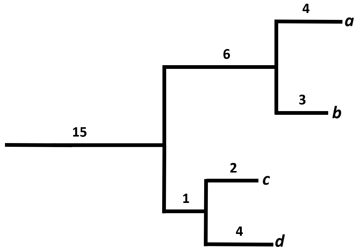
In the case where all four organisms were found in the same sample, the PD would be calculated as:
\[ PD = 15 + 6 + 4 + 3 + 1 + 2 + 4 = 35 \]
If organism a was lost, the PD would be decreased with 4 units to a value of 31. A higher PD is thus indicative of a higher diversity.
Beta diversity describes the between-sample diversity. The diversity can be calculated in different ways, and the choice of method is dependent on the data and the question at hand. Common methods include Bray-Curtis dissimilarity, UniFrac Distance, and Jaccard similarity index (sometimes called Jaccard similarity coefficient).
A crude way to calculate beta diversity is to simply count the number of organisms which exists in one sample, but not the other. The mathematical expression is:
\[ \beta = (\alpha_{sample_{1}} - c) + (\alpha_{sample_{2}} - c) \]
Where \(\alpha_{sample_{1}}\) and \(\alpha_{sample_{2}}\) are the number of unique organisms in sample 1 and 2 (the richness), respectively. \(c\) is the number of organisms which exists in both samples. As the number of shared organisms are subtracted from the richness for each sample, the resulting value is the number of unique organisms in each sample, and the sum increases with the number of unique organisms in the two samples. Ultimately, this means a high value of \(\beta\) indicates a high dissimilarity, i.e. a high diversity.
As an example, consider the following two samples (the top two rows of the test set):
count_matrix_test |>
  slice_head(n = 2)
# A tibble: 2 × 5
Sample Actinomyces Adlercreutzia Agathobacter Akkermansia
<chr> <int> <int> <int> <int>
1 SRR14214860 0 11 190 486
2 SRR14214861 0 12 0 5Sample 1 (SRR14214860 ) has a richness of 3 and sample 2 (SRR14214861) has a richness of 2. They share 2 genera. The beta diversity would be calculated as:
\[ \beta = (3 - 2) + (2 - 2) = 1 \]
The Jaccard index is another way to calculate beta diversity where only the presence/absence of an organism is taken into account. It is calculated as the number of shared organisms (intersection) divided by the total number organisms (union) in the two samples. The equation is as follows::
\[ J(A, B) = \frac{|A \cap B|}{|A \cup B|} \]
From the equation we see why it is called a similarity index. The union (denominator) is just the number of observed organisms, and the intersection (numerator) is the number of shared organisms. The Jaccard index then represent the fraction of the observed organisms which were observed in both samples, i.e. the similarity of the two samples. The value ranges from 0 to 1, where 0 indicates that the two samples do not share any organisms, and 1 indicates that the two samples share the exact same organisms.
When comparing the two first samples in the subset, it is apparent that they share 2 genera, and a total of 3 genera is present between the two samples. The calculation gives:
\[ J(SRR14214860, SRR14214861) = \frac{2}{3} \approx 0.67 \]
To calculate the Jaccard index by using the vegan package, the argument binary is set to TRUE to indicate that the data is binary, i.e. presence/absence of organisms instead of abundance. It is also important to note, that the vegan package actually calculates the dissimilarities, \(1 - \frac{|A \cap B|}{|A \cup B|}\) so a higher value indicates a higher dissimilarity. The Jaccard index is calculated for the test data as follows:
count_matrix_test |>
  slice_head(n = 2) |>
  column_to_rownames(var = "Sample")|>
  vegdist(method = "jaccard",
          binary = TRUE)
SRR14214860
SRR14214861 0.3333333The result is in agreement with the manual calculation since the vegan package calculates the dissimilarity. When inspecting the two samples, they also appear somewhat similar, as the majority of the organisms are present in both sample (even though talking about a majority is a bit misleading when only four organisms are compared). The abundances of the organisms are quite different, and to take that into account, another method is needed.
This measure is widely used to calculate beta diversity. Bray-Curtis dissimilarity takes the composition and abundance of the two compared samples into account. It is also important to note that it is a dissimilarity measure, so a higher value indicates a higher dissimilarity. The value ranges from 0 to 1. A value of 0 indicates that the two samples are identical, while a value of 1 indicates that the two samples do not share any organisms. The metric is calculated as:
\[ BC_{jk} = \frac{\sum_{i=1}^{R} |S_{ij} - S_{ik}|}{\sum_{i=1}^{R} (S_{ij} + S_{ik})} \]
Where \(S_{ij}\) and \(S_{ik}\) are the abundances of the \(i\)’th organism in sample \(j\) and \(k\), respectively. \(R\) is the number of organisms (Bray and Curtis 1957). With the test data, the Bray-Curtis dissimilarity is calculated as follows:
\[ BC_{SRR14214860, SRR14214861} = \frac{|0 - 0| + |11 - 12| + |190 - 0| + |486 - 5|} {(0 + 0) + (11 + 12) + (190 + 0) + (486 + 5)} = 0.955 \]
By using the vegan package the Bray-Curtis dissimilarity can be calculated as follows:
count_matrix_test |>
  slice_head(n = 2) |>
  column_to_rownames(var = "Sample")|>
  vegdist(method = "bray")
SRR14214860
SRR14214861 0.9545455The results are in agreement. The value is close to 1, indicating a high dissimilarity between the two samples. Interestingly, this is a different find compared to the Jaccard index, which indicated a higher similarity between the two samples. The abundances of the organisms in the two samples are quite different, and the Bray-Curtis dissimilarity takes that into account.
The method is based on the phylogenetic tree of the organisms and thereby take the phylogenetic distances into account. UniFrac is shorthand notation for Unique Fraction and is calculated as the sum of unique branch lengths in the phylogenetic tree over the sum of shared branch lengths:
\[ U = \frac{sum \; of \; unique \; branches' \; length}{sum \; of \; all \; branches' \; length} \]
The possible values range from 0 to 1. In the case where the two compared samples share all organisms, the value of the numerator would sum to 0, and the UniFrac would be 0. If the two samples do not share any organisms, the value of the numerator would sum to the total length of the phylogenetic tree (the denominator), and the UniFrac would be 1.
Imagine a phylogenetic tree made from two samples, red and blue. Four different organisms were found in total as seen in the below figure. A red colour indicate an organism found in the red sample, a blue colour indicate an organism found in the blue sample and a purple colour indicate an organism was found in both samples.
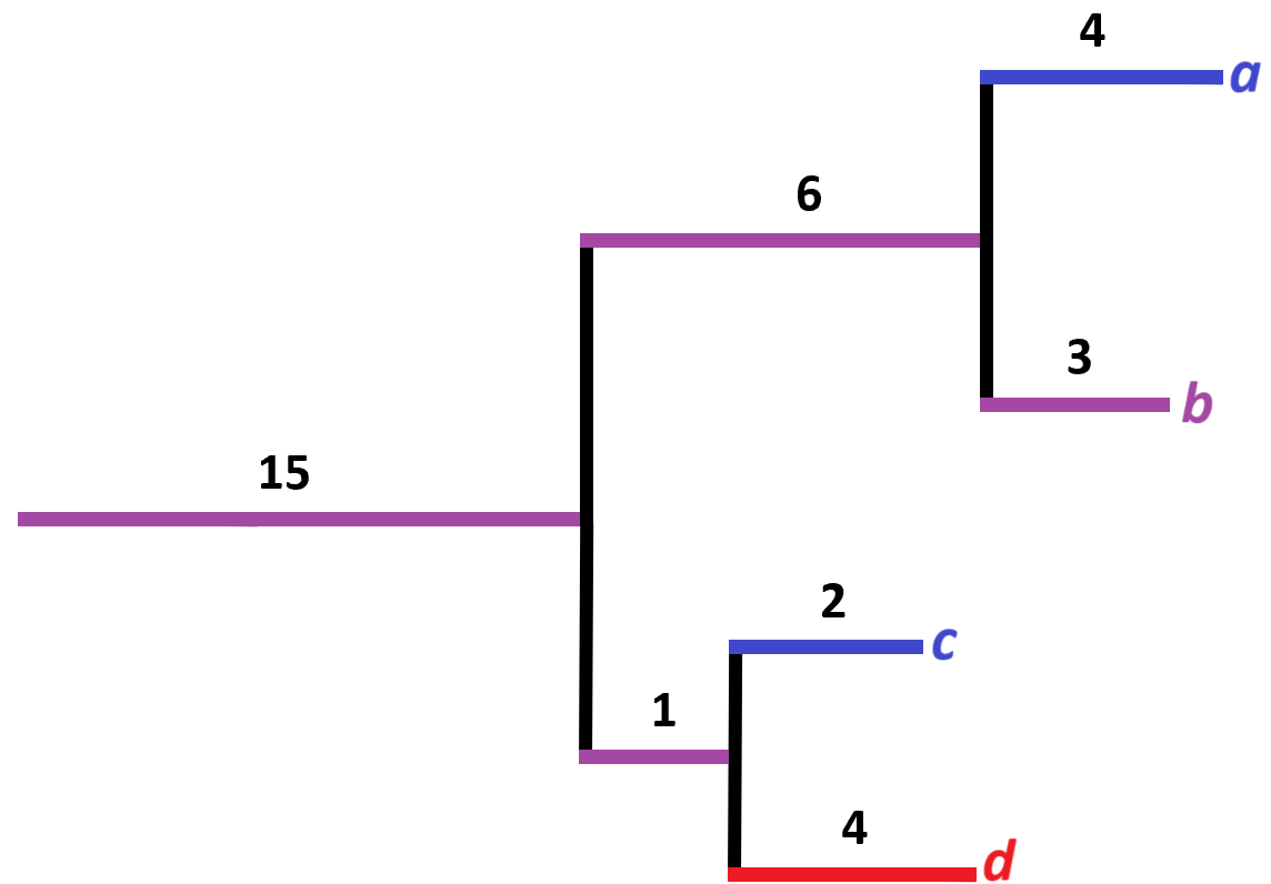
Following the equation above, the UniFrac distance would be calculated as:
\[ U = \frac{4 + 2 + 4}{15 + 6 + 4 + 3 + 1 + 2 + 4} = 0.286 \]
The value indicates that the blue and red samples are quite similar.
The method is divided into two different types, unweighted and weighted. It is the unweighted method which is described above. The weighted method takes the abundance of the organisms into account. The weighted method biases towards the most abundant organisms, while the unweighted method biases more towards the rare organisms. A third version exists, called Generalized UniFrac. This metric has another parameter, usually called \(\alpha\), which can be used to control the balance between the unweighted and weighted methods.
sessioninfo::session_info()─ Session info ───────────────────────────────────────────────────────────────
setting value
version R version 4.3.3 (2024-02-29 ucrt)
os Windows 11 x64 (build 22631)
system x86_64, mingw32
ui RTerm
language (EN)
collate English_United Kingdom.utf8
ctype English_United Kingdom.utf8
tz Europe/Copenhagen
date 2024-05-30
pandoc 3.1.11 @ C:/Program Files/RStudio/resources/app/bin/quarto/bin/tools/ (via rmarkdown)
─ Packages ───────────────────────────────────────────────────────────────────
package * version date (UTC) lib source
backports 1.4.1 2021-12-13 [1] CRAN (R 4.3.1)
broom * 1.0.5 2023-06-09 [1] CRAN (R 4.3.3)
cachem 1.0.8 2023-05-01 [1] CRAN (R 4.3.3)
class 7.3-22 2023-05-03 [2] CRAN (R 4.3.3)
cli 3.6.2 2023-12-11 [1] CRAN (R 4.3.3)
cluster 2.1.6 2023-12-01 [2] CRAN (R 4.3.3)
codetools 0.2-19 2023-02-01 [2] CRAN (R 4.3.3)
colorspace 2.1-0 2023-01-23 [1] CRAN (R 4.3.3)
conflicted 1.2.0 2023-02-01 [1] CRAN (R 4.3.3)
data.table 1.15.4 2024-03-30 [1] CRAN (R 4.3.3)
dials * 1.2.1 2024-02-22 [1] CRAN (R 4.3.3)
DiceDesign 1.10 2023-12-07 [1] CRAN (R 4.3.3)
digest 0.6.35 2024-03-11 [1] CRAN (R 4.3.3)
dplyr * 1.1.4 2023-11-17 [1] CRAN (R 4.3.2)
evaluate 0.23 2023-11-01 [1] CRAN (R 4.3.3)
fansi 1.0.6 2023-12-08 [1] CRAN (R 4.3.3)
fastmap 1.1.1 2023-02-24 [1] CRAN (R 4.3.3)
foreach 1.5.2 2022-02-02 [1] CRAN (R 4.3.3)
furrr 0.3.1 2022-08-15 [1] CRAN (R 4.3.3)
future 1.33.2 2024-03-26 [1] CRAN (R 4.3.3)
future.apply 1.11.2 2024-03-28 [1] CRAN (R 4.3.3)
generics 0.1.3 2022-07-05 [1] CRAN (R 4.3.3)
ggplot2 * 3.5.1 2024-04-23 [1] CRAN (R 4.3.3)
globals 0.16.3 2024-03-08 [1] CRAN (R 4.3.3)
glue 1.7.0 2024-01-09 [1] CRAN (R 4.3.3)
gower 1.0.1 2022-12-22 [1] CRAN (R 4.3.1)
GPfit 1.0-8 2019-02-08 [1] CRAN (R 4.3.3)
gtable 0.3.5 2024-04-22 [1] CRAN (R 4.3.3)
hardhat 1.3.1 2024-02-02 [1] CRAN (R 4.3.3)
hms 1.1.3 2023-03-21 [1] CRAN (R 4.3.3)
htmltools 0.5.8.1 2024-04-04 [1] CRAN (R 4.3.3)
htmlwidgets 1.6.4 2023-12-06 [1] CRAN (R 4.3.3)
infer * 1.0.7 2024-03-25 [1] CRAN (R 4.3.3)
ipred 0.9-14 2023-03-09 [1] CRAN (R 4.3.3)
iterators 1.0.14 2022-02-05 [1] CRAN (R 4.3.3)
jsonlite 1.8.8 2023-12-04 [1] CRAN (R 4.3.3)
knitr 1.46 2024-04-06 [1] CRAN (R 4.3.3)
lattice * 0.22-5 2023-10-24 [2] CRAN (R 4.3.3)
lava 1.8.0 2024-03-05 [1] CRAN (R 4.3.3)
lhs 1.1.6 2022-12-17 [1] CRAN (R 4.3.3)
lifecycle 1.0.4 2023-11-07 [1] CRAN (R 4.3.3)
listenv 0.9.1 2024-01-29 [1] CRAN (R 4.3.3)
lubridate 1.9.3 2023-09-27 [1] CRAN (R 4.3.3)
magrittr 2.0.3 2022-03-30 [1] CRAN (R 4.3.3)
MASS 7.3-60.0.1 2024-01-13 [2] CRAN (R 4.3.3)
Matrix 1.6-5 2024-01-11 [2] CRAN (R 4.3.3)
memoise 2.0.1 2021-11-26 [1] CRAN (R 4.3.3)
mgcv 1.9-1 2023-12-21 [2] CRAN (R 4.3.3)
modeldata * 1.3.0 2024-01-21 [1] CRAN (R 4.3.3)
munsell 0.5.1 2024-04-01 [1] CRAN (R 4.3.3)
nlme 3.1-164 2023-11-27 [2] CRAN (R 4.3.3)
nnet 7.3-19 2023-05-03 [2] CRAN (R 4.3.3)
parallelly 1.37.1 2024-02-29 [1] CRAN (R 4.3.3)
parsnip * 1.2.1 2024-03-22 [1] CRAN (R 4.3.3)
permute * 0.9-7 2022-01-27 [1] CRAN (R 4.3.3)
pillar 1.9.0 2023-03-22 [1] CRAN (R 4.3.3)
pkgconfig 2.0.3 2019-09-22 [1] CRAN (R 4.3.3)
prodlim 2023.08.28 2023-08-28 [1] CRAN (R 4.3.3)
purrr * 1.0.2 2023-08-10 [1] CRAN (R 4.3.3)
R6 2.5.1 2021-08-19 [1] CRAN (R 4.3.3)
Rcpp 1.0.12 2024-01-09 [1] CRAN (R 4.3.3)
readr 2.1.5 2024-01-10 [1] CRAN (R 4.3.3)
recipes * 1.0.10 2024-02-18 [1] CRAN (R 4.3.3)
rlang 1.1.3 2024-01-10 [1] CRAN (R 4.3.3)
rmarkdown 2.26 2024-03-05 [1] CRAN (R 4.3.3)
rpart 4.1.23 2023-12-05 [2] CRAN (R 4.3.3)
rsample * 1.2.1 2024-03-25 [1] CRAN (R 4.3.3)
rstudioapi 0.16.0 2024-03-24 [1] CRAN (R 4.3.3)
scales * 1.3.0 2023-11-28 [1] CRAN (R 4.3.3)
sessioninfo 1.2.2 2021-12-06 [1] CRAN (R 4.3.3)
survival 3.5-8 2024-02-14 [2] CRAN (R 4.3.3)
tibble * 3.2.1 2023-03-20 [1] CRAN (R 4.3.3)
tidymodels * 1.2.0 2024-03-25 [1] CRAN (R 4.3.3)
tidyr * 1.3.1 2024-01-24 [1] CRAN (R 4.3.3)
tidyselect 1.2.1 2024-03-11 [1] CRAN (R 4.3.3)
timechange 0.3.0 2024-01-18 [1] CRAN (R 4.3.3)
timeDate 4032.109 2023-12-14 [1] CRAN (R 4.3.2)
tune * 1.2.1 2024-04-18 [1] CRAN (R 4.3.3)
tzdb 0.4.0 2023-05-12 [1] CRAN (R 4.3.3)
utf8 1.2.4 2023-10-22 [1] CRAN (R 4.3.3)
vctrs 0.6.5 2023-12-01 [1] CRAN (R 4.3.3)
vegan * 2.6-4 2022-10-11 [1] CRAN (R 4.3.3)
withr 3.0.0 2024-01-16 [1] CRAN (R 4.3.3)
workflows * 1.1.4 2024-02-19 [1] CRAN (R 4.3.3)
workflowsets * 1.1.0 2024-03-21 [1] CRAN (R 4.3.3)
xfun 0.43 2024-03-25 [1] CRAN (R 4.3.3)
yaml 2.3.8 2023-12-11 [1] CRAN (R 4.3.2)
yardstick * 1.3.1 2024-03-21 [1] CRAN (R 4.3.3)
[1] C:/Users/Willi/AppData/Local/R/win-library/4.3
[2] C:/Program Files/R/R-4.3.3/library
──────────────────────────────────────────────────────────────────────────────